Lab 4 — Robust summaries & outlier sensitivity

Mean vs. median vs. trimmed mean, and SD vs. MAD, under one contaminating point

Source basis. Original instructor-authored lab; data is synthetic (20 “pipetted volumes” in microliters drawn from a fixed generator, seed 45224). Open texts are conceptual companions cited by section title only (map-don’t-mine); no prose, figures, examples, or exercises are reproduced. See Open readings & attribution. Ungraded — Blackboard is authoritative for graded work.

This lab. Week 10 asked what is fragile in a summary? Here you do it by hand. One reading in a batch of 20 gets mis-transcribed, and you watch three “typical value” summaries — the mean, the median, and the 10% trimmed mean — react to it, then do the same for two measures of spread, the standard deviation and the MAD-based robust scale. The through-line: a robust summary resists a single bad point by design, and knowing how much corruption each one absorbs (its breakdown point) is more useful than any outlier-deletion reflex.

Learning goals

By the end of this lab you should be able to:

Compute and compare the mean, median, and 10% trimmed mean of a sample, and predict which ones a single extreme point can move.
State the breakdown point of a summary — the smallest fraction of the data that can drag it arbitrarily far — and read it off a picture.
Compare the standard deviation with a robust scale (\(1.4826 \times \text{MAD}\)) and explain why one inflates under contamination while the other barely moves.
Say why “see an outlier, delete it” is the wrong default, and what to do instead.

Where we are

A summary is robust if a small amount of bad data cannot move it far. That is not a vague virtue — it is a measurable property. Our setting is deliberately small so you can check every number by hand: a technician records 20 pipetted volumes (target 100 µL). Nineteen readings are clean; the twentieth was meant to be 97.5 µL but was keyed in as 190 µL — a plausible decimal or transcription slip.

The mean of \(n\) numbers is \(\bar{x} = \frac{1}{n}\sum_i x_i\); move one point by \(\Delta\) and the mean moves by exactly \(\Delta/n\), with no ceiling. The median and the trimmed mean throw away — or refuse to chase — extreme values, so a single wild point cannot take them anywhere. The first figure makes that concrete by letting the one suspect reading slide across a wide range while the other nineteen stay put.

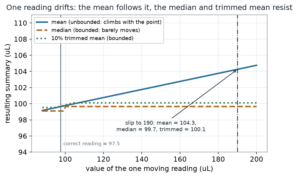
Line plot with the value of one moving reading on the x-axis (88 to 200 microliters) and the resulting summary on the y-axis. A solid mean line climbs steadily from about 99 to 105; a dashed median line and a dotted trimmed-mean line stay flat near 99.7 and 100.1. A vertical guide marks the correct reading at 97.5 and another marks the slip at 190.

What to notice. The mean is a lever: one point at 190 pulls it from 99.6 up to 104.3, and it would keep climbing if the slip were larger. The median and trimmed mean are bounded — they moved by less than a microliter. Robustness here is not luck; the median only cares about the rank of the middle value, and the trimmed mean has already discarded the extremes before averaging.

The one moving reading, as numbers (nonvisual equivalent).

Summary	At the correct reading (97.5 µL)	At the slip (190 µL)
Mean	99.6	104.3
Median	99.1	99.7
10% trimmed mean	99.7	100.1

The R you would run is short — and notice there is no plotting in it; the picture is downstream:

# 20 recorded pipetted volumes (uL); the 20th slipped from 97.5 to 190
volumes <- c(93.0, 95.0, 96.2, 96.5, 97.2, 97.6, 97.8, 98.1, 99.1, 99.1,
             100.2, 100.6, 101.5, 102.5, 103.5, 103.6, 104.0, 104.2, 105.5, 190.0)
x <- volumes
mean(x)               # 104.3 -- pulled up by the slip
median(x)             # 99.7  -- resistant
mean(x, trim = 0.10)  # 100.1 -- 10% trimmed mean, also resistant

Worked example — how much corruption does each summary absorb?

The breakdown point of a summary is the smallest fraction of the sample you must corrupt to send the summary to \(\pm\infty\). It is the honest way to rank robustness. To measure it, corrupt the largest readings one at a time — set each to a huge value — and watch when each summary “flies off.”

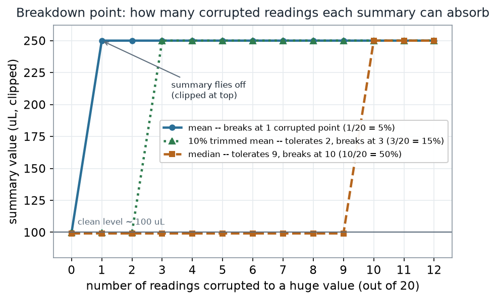
Line plot with the number of readings corrupted to a huge value on the x-axis (0 to 12 of 20) and the resulting summary value on the y-axis, clipped at 250. The solid mean curve jumps to the ceiling at one corrupted point; the dotted trimmed-mean curve stays flat until three corrupted points then jumps; the dashed median curve stays flat until ten corrupted points then jumps.

What to notice. The three curves are flat-then-cliff, and the cliff location is the breakdown point. The mean’s cliff is at one point — on these 20 readings that is 1/20 = 5%, essentially 0% for a large sample. The 10% trimmed mean protects itself up to its trim fraction: it tolerates 2 of 20 and breaks at the 3rd, so 3/20 = 15% here (its nominal breakdown point is the 10% trim fraction). The median holds until half the data is corrupted, the best any summary of location can do — 10/20 = 50%. More trimming buys more protection, at the cost of using less of the data.

Breakdown, as numbers (nonvisual equivalent).

Summary	Corrupted readings absorbed (of 20)	Breakdown point (on this \(n = 20\) sample)
Mean	0 (breaks at the 1st)	1/20 = 5% (≈ 0% for large \(n\))
10% trimmed mean	2 (breaks at the 3rd)	3/20 = 15% (nominal 10%)
Median	9 (breaks at the 10th)	10/20 = 50%

# corrupt the k largest readings to a huge value, then recompute each summary
corrupt <- function(x, k, big = 1e5) {
  i <- order(x, decreasing = TRUE)[seq_len(k)]
  x[i] <- big
  x
}
sapply(0:12, function(k) c(mean   = mean(corrupt(x, k)),
                           median = median(corrupt(x, k)),
                           trim10 = mean(corrupt(x, k), trim = 0.10)))

Spread is fragile too: SD vs. the MAD-based scale

The same lesson applies to spread. The standard deviation squares every deviation, so one far-out point dominates it. A robust alternative is the median absolute deviation, \(\text{MAD} = \text{median}(|x_i - \text{median}(x)|)\), scaled by 1.4826 so that it estimates the same thing as the SD when the data really are Normal. (R’s mad() applies that constant for you.)

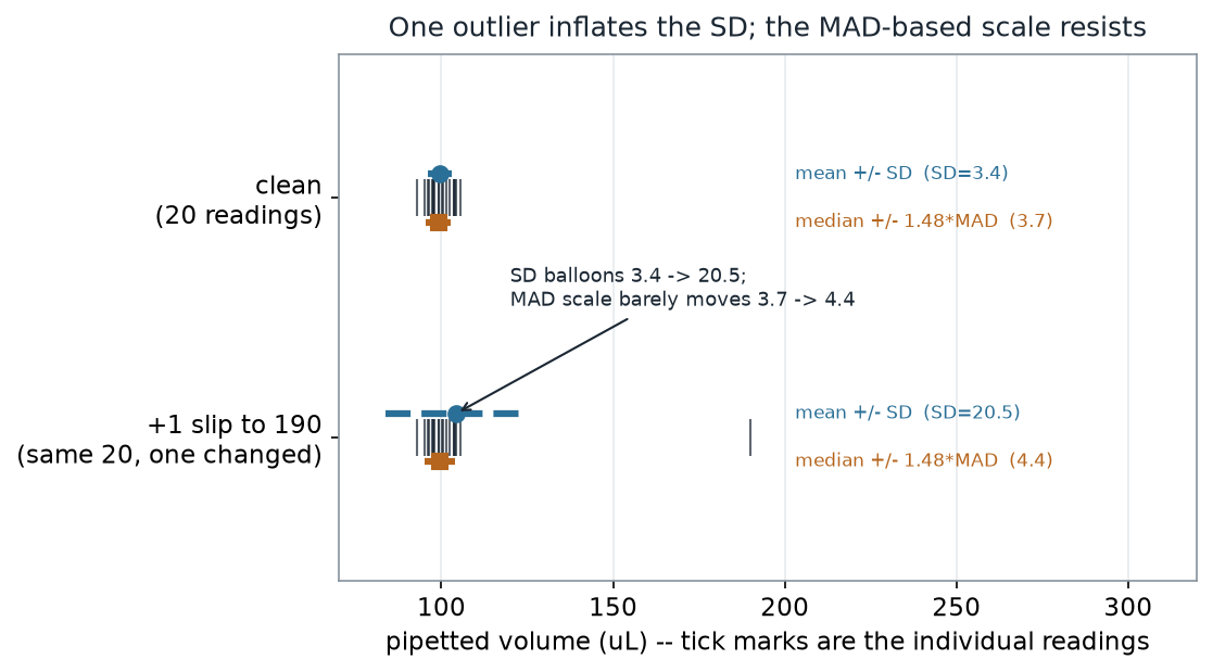
Strip plot with two rows of the same 20 readings — clean on top, one reading slipped to 190 on the bottom. Each row shows a mean plus-or-minus SD interval and a median plus-or-minus 1.48 times MAD interval. On the clean row both intervals are narrow and similar. On the contaminated row the SD interval balloons while the MAD interval stays narrow.

What to notice. One outlier nearly sextupled the SD (3.4 → 20.5) but left the MAD-based scale almost untouched (3.7 → 4.4). If you report “mean ± SD,” a single keystroke error can turn a tight batch into an apparently sloppy one; the robust scale tells you the bulk of the readings are still tightly clustered. On clean data the two agree, so you lose little by defaulting to the resistant pair.

Scale under contamination (nonvisual equivalent).

Scale estimate	Clean (20 readings)	+1 slip to 190 µL
Standard deviation	3.4	20.5
\(1.4826 \times \text{MAD}\)	3.7	4.4

sd(x)   # 20.5 -- inflated by the one slip
mad(x)  # 4.4  -- median absolute deviation, already scaled by 1.4826 in R

A common mistake

“An outlier is an error, so delete it and move on.” Deleting-by-reflex is a decision disguised as housekeeping. The 190 µL point might be a transcription slip — but it might be a real double-dispense worth catching, and quietly dropping it hides the very problem you should report. Robust methods let you keep the point in view and still get a trustworthy summary. Robust ≠ throw data away. Investigate the point, report a resistant summary and a sensitivity check (result with and without it), and say what you did.

Decision diagram. A top box, 'you spot a reading far from the rest (190 uL),' splits into two paths. The left path — auto-delete it, then report mean and SD of the rest — is labeled a fragile habit that discards possibly-real data and hides the recording problem. The right path — investigate whether it is a recording error or a real extreme, then report a robust summary plus the point and a sensitivity check — is labeled the course habit, 'robust does not mean throw data away.' — Decision diagram. A top box, ‘you spot a reading far from the rest (190 uL),’ splits into two paths. The left path — auto-delete it, then report mean and SD of the rest — is labeled a fragile habit that discards possibly-real data and hides the recording problem. The right path — investigate whether it is a recording error or a real extreme, then report a robust summary plus the point and a sensitivity check — is labeled the course habit, ‘robust does not mean throw data away.’

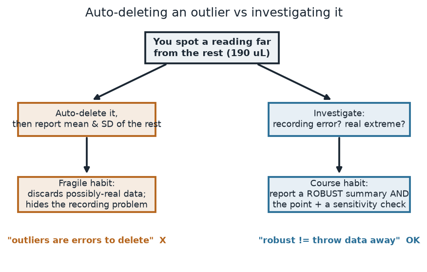
What to notice. The two paths start from the same observation and diverge on habit, not on evidence. Robust summaries make the honest path cheap: you do not have to decide whether the point is “allowed to stay” before you can report a stable number.

The two paths, as text (nonvisual equivalent).

Reflex (fragile)	Course habit
Auto-delete the point, report mean ± SD of the rest	Investigate: recording error or real extreme?
Discards possibly-real data; hides the problem	Report a robust summary and the point + a sensitivity check

Check your understanding (ungraded)

Moving one reading by \(\Delta\) moves the mean by exactly \(\Delta/n\). Using \(n = 20\), by how much would the mean move if the slip had been to 290 µL instead of 190? Would the median change?
In your own words, what does a breakdown point of 50% promise, and why can no summary of location do better?
The 10% trimmed mean absorbed 2 corrupted readings here. If you switched to a 20% trimmed mean on the same 20 readings, how many would it absorb before breaking?
The SD went from 3.4 to 20.5 but the MAD-based scale went from 3.7 to 4.4. Which one would you report to a colleague as “how spread out are the readings,” and what would you say about the 190 µL point?

Reading guide

OpenIntro Statistics 4e — Examining numerical data (center and spread) — a conceptual companion to mean/median and SD; read for the definitions, then verify the resistance claims against the pictures above.
Learning Statistics with R (Navarro) — Descriptive statistics — reinforces the trimmed mean and the median absolute deviation as everyday robust summaries (cited, not reproduced).
NIST/SEMATECH e-Handbook — What are outliers and how do we detect them? — an instructor reference on treating outliers as something to investigate, not automatically delete.

Accessibility notes

Mathematics is live text (\(\bar{x}=\frac{1}{n}\sum_i x_i\) and \(1.4826\times\text{MAD}\) render as MathML, not images). Every figure carries an alt line stating its message, a “what to notice” reading, and an adjacent data-summary table, so each point survives without the picture. Series are distinguished by linestyle and marker (mean = solid/circle, median = dashed/square, trimmed mean = dotted/triangle) and by value-bearing labels, never color alone. A clean lint and a clean render are evidence; the rendered assistive-technology review is a human step.

Assessment (descriptive only)

This lab contributes learning evidence toward choosing and defending a robust summary and reading a breakdown point. That is the shape only; the actual graded prompts, points, and due dates live in Blackboard.

Public vs. graded. These are public, ungraded notes and practice. Graded prompts, keys, rubrics, point values, and due dates live in Blackboard Ultra, which governs.

Looking ahead

Robust summaries generalize to robust models. Week 11 replaces the single mean with a whole regression line and asks the same question one dimension up: when one high-leverage point can swing an ordinary least-squares fit, what does a resistant fit do instead — and what is its breakdown point?