Lab 3 — Rank methods, hands-on
Build a Wilcoxon signed-rank test and a rank-sum test from the ranks up
Source basis. Original instructor-authored lab; all data is synthetic — two small product-team experiments drawn from a fixed generator (seed 45223). Open texts are conceptual companions cited by section title only (map-don’t-mine); no prose, figures, examples, or exercises are reproduced. See Open readings & attribution. Ungraded — Blackboard is authoritative for graded work.
This lab. Weeks 7 and 8 introduced the two workhorse rank tests: the Wilcoxon signed-rank test for matched pairs and the Wilcoxon rank-sum / Mann–Whitney test for two independent groups. Here you build both by hand — rank, sum, and shuffle — on two synthetic mini-experiments, then watch what ties do to the null and what happens when you run the wrong test on the right data. The whole point is that a rank test is only as good as the match between its null and your study’s structure.
Learning goals
By the end of this lab you should be able to:
- Reduce matched pairs to within-pair differences, rank the absolute differences (averaging ties), and compute the signed-rank statistic \(W^{+}\).
- Pool two independent groups, rank all values together, sum one group’s ranks to get \(W\), and build its permutation null by shuffling labels.
- Explain how tied values get averaged ranks and how that coarsens (and slightly narrows) the null.
- Recognize a paired-vs-independent mismatch — running a two-sample test on paired data — as a real error that costs you power, not a stylistic choice.
Where we are
Our recurring question is what is fragile here, and what can we still say? A rank test answers the second half cheaply: throw away the raw distances, keep only the ordering, and no single wild value can drag the conclusion around. But the ranking machinery has to be matched to how the data were collected. Paired data carries structure — the same unit measured twice — that a two-sample test cannot see. So we work through both tests on their own data, then put the mismatch under a microscope.
Part 1 — paired data: the signed-rank test
Ten analysts each rated a dashboard’s usability on a 0–100 scale before and after a redesign. Each analyst is their own control, so the quantity that matters is the within-analyst difference, \(d_i = \text{after}_i - \text{before}_i\). Eight analysts rated the redesign higher; two rated it slightly lower. To run the signed-rank test we rank the absolute differences from smallest to largest, then add up the ranks that belong to positive differences — that sum is \(W^{+}\).
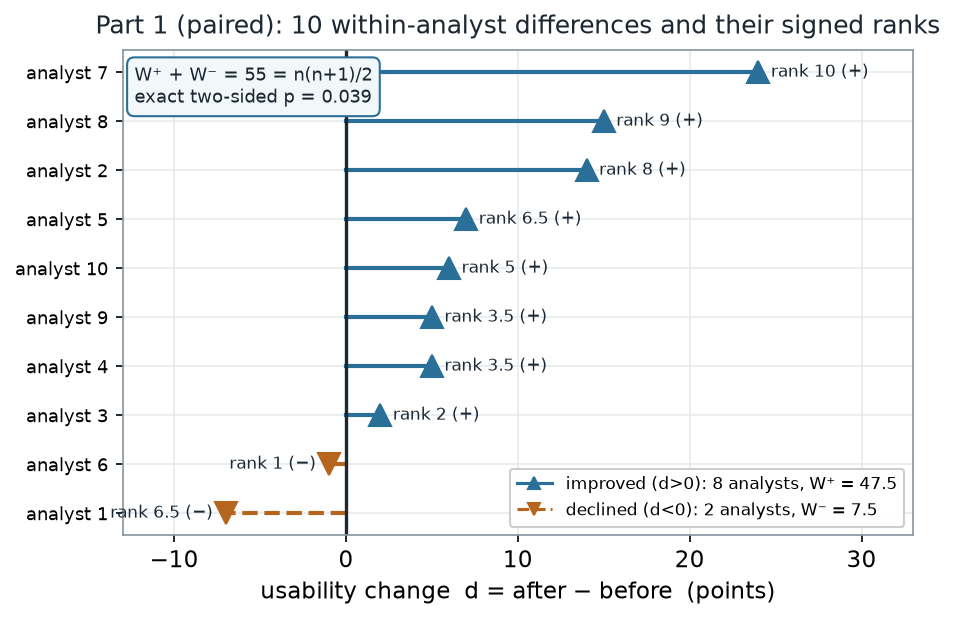
What to notice. Only two of the ten changes are declines — one tiny (−1, rank 1) and one moderate (−7, whose magnitude ties a +7 and so earns the middling rank 6.5) — so together they contribute just \(W^{-} = 7.5\). It is the count of declines, not their being small, that keeps \(W^{-}\) low: rank 6.5 sits right in the middle of a ten-item ranking. The eight improvements, several of them large, carry the rest: \(W^{+} = 47.5\). The two sums are locked together at \(W^{+} + W^{-} = n(n+1)/2 = 55\) before you compute either one, which is a handy arithmetic check. Signs are shown by marker shape (▲ vs ▼) and stem direction, never color alone.
The paired differences, as numbers (nonvisual equivalent).
| Quantity | Value |
|---|---|
| \(n\) pairs | 10 |
| Differences \(d\) (after − before), sorted | −7, −1, +2, +5, +5, +6, +7, +14, +15, +24 |
| Positive · negative · zero | 8 · 2 · 0 |
| \(\lvert d\rvert\) ranked (ties averaged) | 1, 2, 3.5, 3.5, 5, 6.5, 6.5, 8, 9, 10 |
| \(W^{+}\) (sum of positive-difference ranks) | 47.5 |
| \(W^{-}\) (sum of negative-difference ranks) | 7.5 |
| \(W^{+} + W^{-} = n(n+1)/2\) | 55 |
| Exact two-sided \(p\) | 0.039 |
Worked example — building \(W^{+}\) from scratch
The whole test is four lines of R, and — as always in this course — there is no plotting in it; the picture above is a static PNG the lab ships:
before <- c(57, 48, 43, 50, 53, 49, 43, 54, 40, 38)
after  <- c(50, 62, 45, 55, 60, 48, 67, 69, 45, 44)
d <- after - before          # 10 within-analyst differences
r <- rank(abs(d))            # rank |d|; ties (two 5s, two 7s) share the average rank
Wplus <- sum(r[d > 0])       # signed-rank statistic W+ = 47.5

# EXACT two-sided p: enumerate all 2^10 = 1024 equally-likely sign patterns of the ranks
# (this is what "exact" means, and it uses the averaged tied ranks directly).
signs   <- as.matrix(expand.grid(rep(list(c(0, 1)), length(r))))   # 1024 x 10
Wnull   <- as.numeric(signs %*% r)                                 # W+ under each sign pattern
p_exact <- mean(abs(Wnull - sum(r) / 2) >= abs(Wplus - sum(r) / 2))  # 0.039

# Base R CANNOT give the exact p here: with ties it warns and falls back to the normal
# approximation (a different number), so `exact = TRUE` does not enumerate as above.
wilcox.test(after, before, paired = TRUE)   # normal approx (continuity-corrected), NOT the exact 0.039
Two absolute differences tie at 5 and two tie at 7. Tied magnitudes share the average of the ranks they would have occupied: the two values of 5 would sit at ranks 3 and 4, so both become 3.5; the two values of 7 would sit at ranks 6 and 7, so both become 6.5. Averaging ties is what keeps the rank total fixed at 55. Because the two declines are the smallest changes, \(W^{+} = 47.5\) lands far above its null mean of 27.5, and enumerating all \(2^{10} = 1024\) equally-likely sign patterns puts the exact two-sided \(p\) at 0.039 — evidence, at the 5% level, that the redesign shifted usability.
Part 2 — two independent groups: the rank-sum test
Now a different, unpaired experiment. Two independent cohorts timed how many minutes they took to finish a setup task: a guided group (\(n_1 = 9\)) with on-screen help, and an unguided group (\(n_2 = 11\)) without it. There is no pairing to exploit, so the rank idea scales up: pool all 20 times, rank them \(1\)–\(20\) (averaging ties), and sum the ranks of the guided group. That sum is \(W = 52.5\). To judge it we shuffle the group labels across the fixed ranks many times and see how far out \(W\) falls.
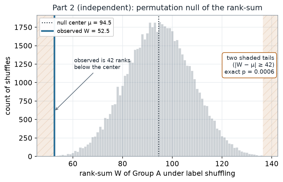
What to notice. The observed rank-sum (\(52.5\)) is far into the lower tail — the guided group collected the low ranks (fast times). Enumerating all \(\binom{20}{9} = 167{,}960\) ways to split the fixed ranks into a size-9 group gives an exact two-sided \(p = 0.0006\): only about six in ten thousand label shuffles land a rank-sum this far from \(94.5\) in either direction. The shaded bands are the rejection region; the observed value sits at the edge of the left one.
The rank-sum read-out (nonvisual equivalent).
| Quantity | Value |
|---|---|
| \(n_1\) (guided) · \(n_2\) (unguided) · \(N\) | 9 · 11 · 20 |
| Median, guided · unguided (minutes) | 6.0 · 14.0 |
| Rank-sum \(W\) (guided) | 52.5 |
| Null center \(\mu_W = n_1(N+1)/2\) | 94.5 |
| Mann–Whitney \(U = W - n_1(n_1{+}1)/2\) | 7.5 |
| \(U/(n_1 n_2)\) = estimate of \(P(\text{guided} > \text{unguided})\) | 0.076 |
| Exact two-sided permutation \(p\) | 0.0006 |
The Mann–Whitney \(U = 7.5\) carries a plain-language reading: of the \(n_1 n_2 = 99\) guided-vs-unguided matchups, the guided user finished slower in only 7.5 of them, so \(U/(n_1 n_2) = 0.076\) estimates \(P(\text{guided} > \text{unguided})\). The guided cohort was faster in roughly 92% of head-to-head comparisons. The R is again short and plotting-free:
guided   <- c(4, 4, 5, 5, 6, 6, 10, 11, 13)               # n1 = 9
unguided <- c(9, 11, 11, 12, 13, 14, 15, 16, 22, 22, 24)  # n2 = 11
r  <- rank(c(guided, unguided))      # pool, rank all 20, average ties
W  <- sum(head(r, length(guided)))   # rank-sum of the guided group = 52.5
mu <- mean(r) * length(guided)       # null mean of W = 94.5

# EXACT two-sided p: enumerate all choose(20, 9) = 167,960 label splits of the fixed ranks.
Wall    <- combn(length(r), length(guided), function(cols) sum(r[cols]))
p_exact <- mean(abs(Wall - mu) >= abs(W - mu))   # exact two-sided p = 0.0006

# The same null by label shuffling (Monte Carlo) -- matches the exact p up to simulation error:
set.seed(45223)
Wnull <- replicate(20000, sum(sample(r, length(guided))))
mean(abs(Wnull - mu) >= abs(W - mu))  # ~ 0.0006 (approximate)

# Base R gives the normal approximation here too (ties -> a warning, not the exact p):
wilcox.test(guided, unguided)         # Mann-Whitney U / rank-sum, normal approx (not exact)
What ties do to the null
Both tests lean on averaging tied ranks, and ties are not cosmetic — they reshape the reference distribution. To see it exactly, take the cleanest possible case: a size-4 group inside \(N = 8\), small enough to enumerate all \(\binom{8}{4} = 70\) label assignments. Compare the null when all eight values are distinct (ranks \(1\)–\(8\)) with the null when four middle values tie (each getting the average rank 4.5).
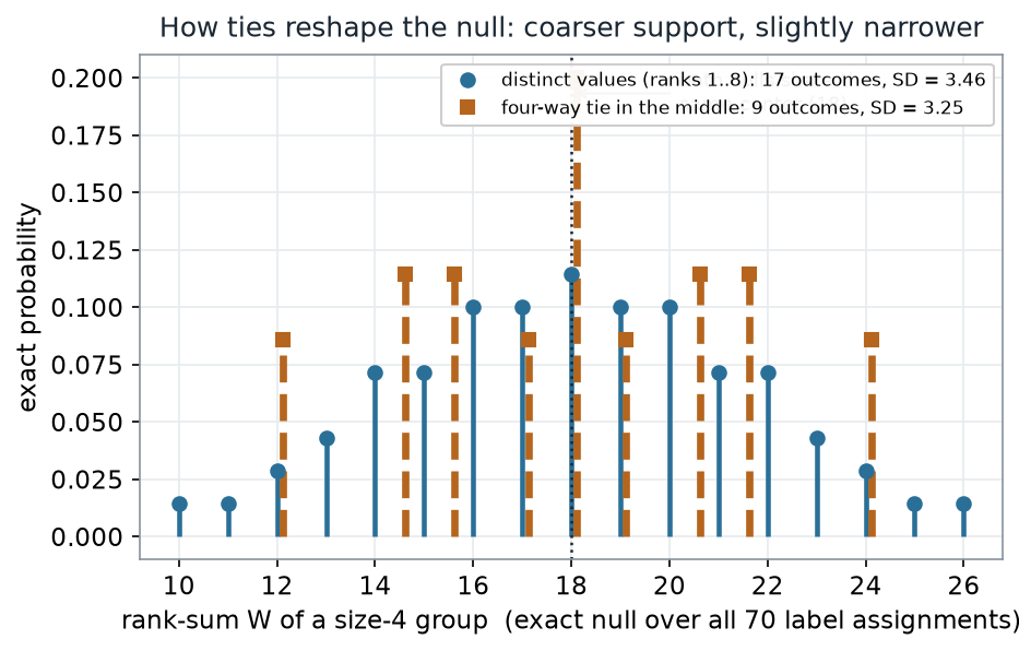
What to notice. Ties do not move the null’s center (both sit at 18), but they collapse many distinct rank-sums onto the same value: the tied null lands on only 9 possible outcomes instead of 17, and its standard deviation drops from 3.46 to 3.25. In this exact, heavily-tied enumeration it is the coarse, heavy-atom support — not the smaller SD — that decides the tail: judging the observed value against the no-tie null (ignoring the ties) reports a \(p\) that is slightly too small here — for instance at \(\lvert W - 18\rvert = 6\) the correct tied \(p\) is 0.171, versus 0.114 from the distinct-value null. The direction is not universal: the usual large-sample normal-approximation tie correction only shrinks the variance (SD 3.25 < 3.46), which by itself makes ignoring ties conservative — a \(p\) slightly too big. So whether ignoring ties helps or hurts depends on whether you read the exact null or the approximation. Distinct and tied nulls are drawn with different markers and linestyles (● solid vs ■ dashed), not color alone.
Ties read-out (nonvisual equivalent).
| Null (size-4 group, \(N=8\)) | Distinct outcomes | SD | Center |
|---|---|---|---|
| Distinct values (ranks 1–8) | 17 | 3.46 | 18 |
| Four-way tie in the middle | 9 | 3.25 | 18 |
The mistake this lab is built to prevent
“A rank test is a rank test — signed-rank or rank-sum, either one is fine.” No. The signed-rank test reads one difference per pair; the rank-sum test reads two independent groups. They resample different nulls and answer different questions. Run the two-sample rank-sum on paired data and you have thrown the pairing away — the very structure that made the study strong — and traded it for a weaker, different test.
Make the cost concrete with the Part 1 data. The correct analysis — the signed-rank test on the ten paired differences — returned \(p = 0.039\). Now do the wrong thing: pretend the ten “before” and ten “after” scores are twenty independent people and run a rank-sum on them.
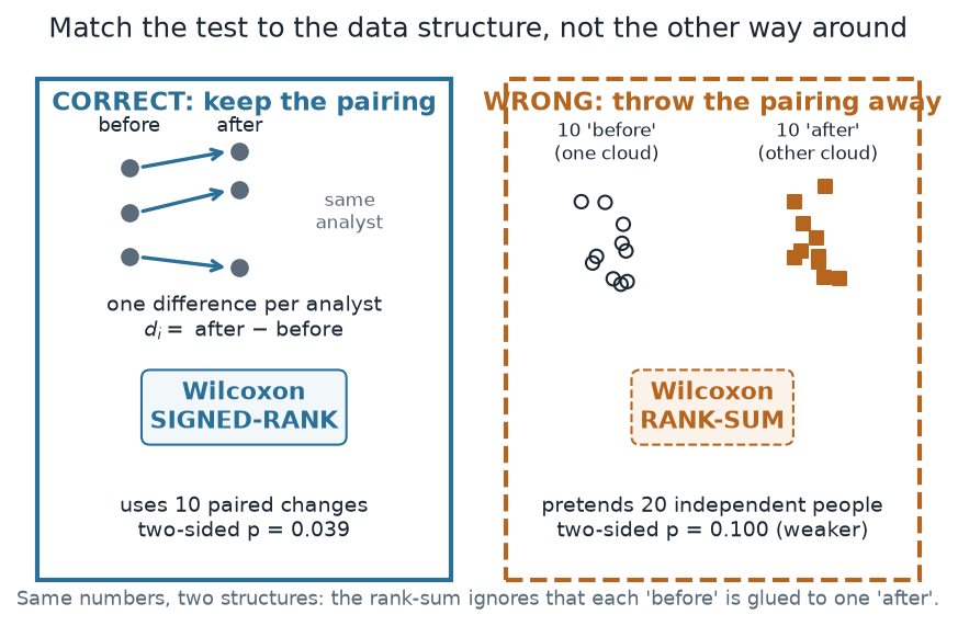
What to notice. Nothing about the numbers changed; only the claimed structure did. The unpaired rank-sum drowns each analyst’s real change in the large spread between analysts (some are harsh raters, some generous), so a genuine effect that the paired test flags at \(p = 0.039\) slips to a non-significant \(p = 0.100\). Unpairing is not a milder analysis — it is usually a weaker one, and it answers a different question.
Right test vs wrong test (nonvisual equivalent).
| Analysis of the Part 1 data | What it uses | Two-sided \(p\) |
|---|---|---|
| Signed-rank (correct) | 10 within-analyst differences | 0.039 |
| Rank-sum (wrong — unpaired) | 10 “before” vs 10 “after” as independent | 0.100 |
Check your understanding (ungraded)
- In Part 1, the two negative differences were −1 and −7. Explain, without recomputing, why they contributed exactly \(W^{-} = 7.5\) and how you could have predicted \(W^{+}\) from that alone.
- Two absolute differences tied at 5 and two tied at 7. Assign their averaged ranks from first principles, and say why averaging (rather than breaking ties arbitrarily) keeps the total at 55.
- In Part 2 the observed rank-sum \(W = 52.5\) sat 42 ranks below the null center of 94.5. Describe in words what the permutation null is a distribution of, and why a rank-sum far from 94.5 counts as evidence.
- The tied null in the ties figure had 9 outcomes and SD 3.25, versus 17 outcomes and SD 3.46 with no ties. For this exact enumeration, which way does judging the observed value against the no-tie null push a two-sided \(p\) — and why does the large-sample normal-approximation tie correction, which only shrinks the variance, push it the other way?
- The unpaired rank-sum on the Part 1 data gave \(p = 0.100\) where the paired test gave \(p = 0.039\). Describe a study where the mismatch would instead make you miss an effect entirely.
Reading guide
- OpenIntro Statistics 4e — inference for paired data — a conceptual companion to reducing pairs to one difference each; read for the framing, then map it onto the signed-rank lollipop above.
- Learning Statistics with R (Navarro) — the Wilcoxon signed-rank test — an instructor reference on ranking \(\lvert d\rvert\) and forming \(W^{+}\) (cited, not reproduced).
- Learning Statistics with R (Navarro) — the Mann–Whitney (rank-sum) test — an instructor reference on pooling, ranking, and the \(U\)–\(W\) correspondence.
- NIST/SEMATECH e-Handbook — Wilcoxon signed rank test — a reference for the exact null and the tie correction you saw reshape the distribution.
Accessibility notes
Mathematics is live text (\(W^{+}\), \(n(n+1)/2\), and \(\binom{20}{9}\) render as MathML, not images). Every figure carries an alt line stating its message, an adjacent “what to notice” reading, and a data-summary table, so each point survives without the picture. Improvements and declines, and distinct versus tied nulls, are distinguished by marker shape and linestyle (▲/● solid vs ▼/■ dashed) and by direct labels, never by color alone. A clean lint and a clean render are evidence; the rendered assistive-technology review is a human step.
Assessment (descriptive only)
This lab contributes learning evidence toward building a rank test from the ranks up and matching the test to the data’s structure. That is the shape only; the actual graded prompts, values, and due dates live in Blackboard.
Public vs. graded. This is a public, ungraded lab and practice. Graded prompts, keys, rubrics, values, and due dates live in Blackboard Ultra, which governs.
Looking ahead
The ranking habit you built here — pool, rank, sum, shuffle — is the same move behind the categorical and ordinal tests coming next, where the “ranks” become counts in a table and an exact permutation null again beats a shaky large-sample approximation when the counts are small.