Lab 2 — Bootstrap confidence intervals
Resample with replacement, read a percentile interval, and find where it disagrees with the t interval
Source basis. Original instructor-authored lab; data is synthetic (45 “food-delivery times” in minutes, drawn from a fixed generator, seed 45222). Open texts are conceptual companions cited by section title only (map-don’t-mine); no prose, figures, examples, or exercises are reproduced. See Open readings & attribution. Ungraded — Blackboard is authoritative for graded work.
This lab. Weeks 5–6 built a bootstrap distribution and turned it into a percentile interval. Here you do it: resample one sample with replacement, read the interval off the tails, hold it up against the textbook \(\bar{x} \pm t\,\text{SE}\) interval, and then stress-test the recipe two ways — does it keep its 95% promise across repeated studies, and how many resamples do you actually need before the interval you report stops wobbling? Run each block in Posit Cloud, then check your output against the target numbers below — the resampling ones are targets to land near, not match to the last decimal (Step 1 says why).
Learning goals
By the end of this lab you should be able to:
- Build a bootstrap distribution of the sample mean and read a percentile interval off its 2.5th and 97.5th percentiles.
- Contrast the percentile interval with the \(\bar{x} \pm t\cdot\text{SE}\) interval and say why they differ on skewed data.
- Interpret coverage as a repeated-sampling property of the procedure, not a probability for one interval.
- Separate two kinds of error: sampling error (fixed by your one sample) from Monte-Carlo error (the bootstrap’s own noise), and choose \(B\) large enough that the second one stops mattering.
Where we are
We keep asking the same question: what is fragile here, and what can we still say? A single sample mean is fragile — draw another sample and it moves. The bootstrap measures that movement by resampling the sample with replacement, and a confidence interval packages the movement into a stated range.
Your data is a batch of 45 synthetic food-delivery times (minutes), right-skewed: a few very long deliveries pull the tail out to the right. Load it and look before you resample.
# the observed sample (synthetic; 45 delivery times, minutes)
delivery_times <- c(2.2, 4.1, 4.1, 4.4, 4.4, 4.8, 5.8, 5.9, 5.9, 6.9, 7.0, 8.5, 8.6, 9.2,
                    10.4, 11.2, 11.4, 11.8, 11.9, 11.9, 12.1, 12.2, 15.4, 16.1, 16.3, 18.5,
                    20.0, 20.0, 20.1, 20.8, 20.8, 21.9, 23.2, 23.3, 26.1, 27.7, 29.4, 30.8,
                    34.1, 35.0, 36.7, 37.2, 41.1, 73.4, 86.1)
length(delivery_times)          # 45
mean(delivery_times)            # 19.3
sd(delivery_times)              # 16.8
quantile(delivery_times)        # min 2.2, Q1 8.5, median 15.4, Q3 23.3, max 86.1
The sample, as numbers (nonvisual equivalent).
| Summary | Value (minutes) |
|---|---|
| n | 45 |
| Min · Q1 · Median · Q3 · Max | 2.2 · 8.5 · 15.4 · 23.3 · 86.1 |
| Mean | 19.3 |
| SD | 16.8 |
Step 1 — Build the percentile interval
The percentile method is almost embarrassingly simple: resample with replacement, recompute the mean each time, collect \(B\) of those bootstrap means, and read off the 2.5th and 97.5th percentiles. Everything between them is the interval — no formula, no normal table, no assumption that the mean is Normally distributed. The R contains no plotting; the picture is downstream.
set.seed(45222)
x    <- delivery_times
B    <- 4000
boot <- replicate(B, mean(sample(x, size = length(x), replace = TRUE)))

quantile(boot, c(0.025, 0.975))   # percentile interval  ->  ~15.0 to 24.5
sd(boot)                          # bootstrap standard error of the mean  ->  ~2.50
Your numbers will land beside these targets, not exactly on them. The printed values come from this course’s figure generator, whose random-number stream is not R’s set.seed(45222), so sample() draws a different sequence of resamples. At \(B = 4000\) the percentile endpoints are reproducible only to about a tenth of a minute — so treat ~15.0 to 24.5 as a target to land near, not a checksum to match. That small gap is exactly the Monte-Carlo wobble you will measure in the last section: it shrinks as \(B\) grows, and it is what makes any two seeds disagree in the last decimal.
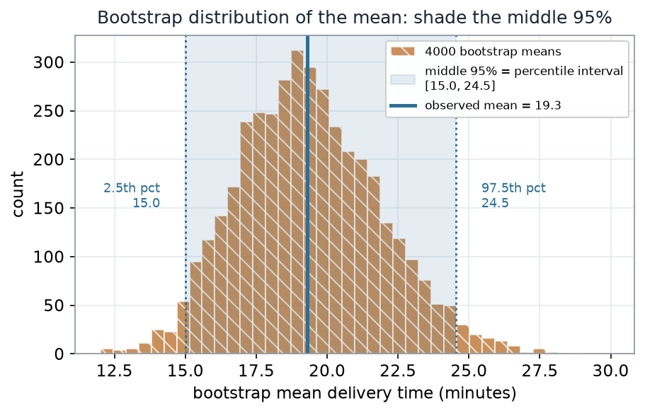
What to notice. The interval is nothing more than the middle 95% of the sorted bootstrap means: 2.5% of the resampled means fall below 15.0 and 2.5% above 24.5. Its edges are two percentiles of a lightly right-skewed pile, so the upper arm (5.2) runs a little longer than the lower arm (4.3). The pipeline never assumed a shape — it read the shape the resamples produced.
Percentile read-out (nonvisual equivalent).
| Quantity | Value |
|---|---|
| Observed mean | 19.3 min |
| Bootstrap SE of the mean | 2.50 min |
| Percentile interval (2.5th, 97.5th) | [15.0, 24.5] |
| Lower arm · upper arm (about the mean) | 4.3 · 5.2 |
| Resamples (\(B\)) | 4000 |
Step 2 — Compare with the t interval
The textbook interval is \(\bar{x} \pm t_{0.975,\,n-1}\cdot\text{SE}\), with \(\text{SE} = s/\sqrt{n}\). By construction it is symmetric — the same distance left and right of \(\bar{x}\). The percentile interval is free to be asymmetric, so on skewed data the two disagree.
n  <- length(x)
se <- sd(x) / sqrt(n)
mean(x) + c(-1, 1) * qt(0.975, df = n - 1) * se   # t interval  ->  14.3 to 24.4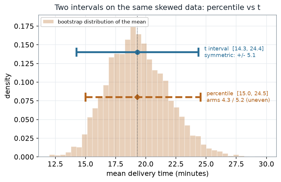
What to notice. The \(t\) interval reaches down to 14.3 because it is forced to be symmetric — it spends the same 5.1 minutes on each side of \(\bar{x}\). The percentile interval only reaches 15.0 on the low side, because the bootstrap means do not stretch as far left as a symmetric rule assumes. The percentile method lets the data’s shape set the shape of the interval; the \(t\) method imposes a symmetric one. Here the two are close — but the gap widens as skew grows and \(n\) shrinks.
Two intervals side by side (nonvisual equivalent).
| Interval | Lower | Upper | Half-width / arms | Symmetric? |
|---|---|---|---|---|
| \(t\): \(\bar{x} \pm t\cdot\text{SE}\) (\(t_{0.975,44}=2.0154\)) | 14.3 | 24.4 | \(\pm 5.1\) | yes |
| Percentile (2.5th, 97.5th) | 15.0 | 24.5 | 4.3 / 5.2 | no |
Step 3 — Does the interval keep its promise?
“95% confidence” is a claim about the procedure, not about the one interval you got. Because the data is synthetic we know the true mean is exactly 20, so we can do the experiment you can never do in practice: repeat the whole study many times and watch the intervals. Each repeat draws a fresh sample, bootstraps it, and forms a percentile interval; then we count how many capture 20.
# one repeat of the WHOLE study -> a fresh percentile interval (schematic; the picture is downstream)
one_ci <- function() {
  s <- rgamma(45, shape = 2, scale = 10)          # a fresh sample from the known population
  quantile(replicate(1000, mean(sample(s, replace = TRUE))), c(0.025, 0.975))
}
# repeat one_ci() many times and record the share of intervals that contain 20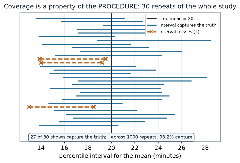
What to notice. Every repeat produces a different interval, because each starts from a different sample. “95% confidence” is a promise about the long-run share that capture the truth, read off the collection of intervals — not any single one. Notice too that the share came out 93.2%, a little short of 95%: for the mean of skewed data at this \(n\), the percentile interval mildly undercovers.
Coverage read-out (nonvisual equivalent).
| Quantity | Value |
|---|---|
| True mean (known, synthetic) | 20 min |
| Repeats simulated | 1000 |
| Intervals capturing the truth | 93.2% |
| Shown in the figure | 27 of 30 capture |
A common mistake
“Any number of resamples is fine — bootstrap is bootstrap.” Not quite. There are two sources of error here, and they behave differently. Sampling error is baked into your one sample; more resamples cannot touch it. Monte-Carlo error is the bootstrap’s own randomness — and it shrinks as you raise \(B\). Report an interval from too few resamples and the endpoints you publish are themselves noisy: rerun with a new seed and they move. The fix is not more data, it is more \(B\).
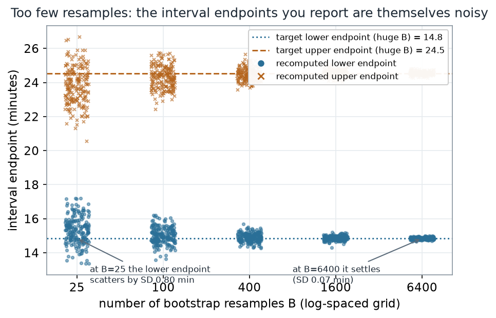
What to notice. The scatter is pure Monte-Carlo noise: the sample never changed, only the number of resamples did. At \(B = 25\) the reported endpoints wander by nearly a minute; at \(B = 6400\) they barely move. That is why the default \(B\) in this course is in the thousands — large enough that the interval you report is the sample’s interval, not the random-number generator’s.
Resample-count read-out (nonvisual equivalent).
| Quantity | Value |
|---|---|
| Recomputes per grid point | 200 |
| Lower-endpoint SD at \(B = 25\) | 0.80 min |
| Lower-endpoint SD at \(B = 6400\) | 0.07 min |
| Target interval (very large \(B\)) | [14.8, 24.5] |
Check your understanding (ungraded)
- In one sentence, describe how to turn a bootstrap distribution of the mean into a percentile interval — what two numbers do you read off, and from what?
- The percentile interval reached down to 15.0 while the \(t\) interval reached 14.3. Explain the difference in terms of the shape of the bootstrap distribution.
- A classmate says “the interval \([15.0, 24.5]\) has a 95% chance of containing the mean.” Rewrite the claim so it is correct, and connect it to the 93.2% you measured.
- You rerun the bootstrap with a new seed and get \([15.1, 24.3]\) instead of \([15.0, 24.5]\). Which kind of error moved the endpoints — sampling or Monte-Carlo — and what single change makes it smaller?
Reading guide
- IMS — Bootstrap confidence intervals — a conceptual companion to reading an interval off a bootstrap distribution; read for the intuition, then check it against the pictures above.
- ModernDive — Bootstrapping and confidence intervals — reinforces the percentile method and the repeated-sampling meaning of a confidence level.
- OpenIntro Statistics 4e — Confidence intervals — the \(\bar{x}\pm t\cdot\text{SE}\) interval we contrast against, for a common reference point.
- NIST/SEMATECH e-Handbook — Bootstrap uncertainty — an instructor reference on bootstrap interval methods and how many resamples they need (cited, not reproduced).
Accessibility notes
Mathematics is live text (\(\bar{x} \pm t\cdot\text{SE}\) renders as MathML, not an image). Every figure carries an alt line stating its message, a “what to notice” reading, and an adjacent data-summary table, so each point survives without the picture. Series are distinguished by linestyle and marker (solid = the \(t\) interval / a capturing interval / the target-lower line; dashed with an “×” = the percentile interval / a missing interval; dots vs. × for lower vs. upper endpoints) and by labels, not color alone. A clean lint and a clean render are evidence; the rendered assistive-technology review is a human step.
Assessment (descriptive only)
This lab contributes learning evidence toward constructing and reading a percentile confidence interval, contrasting it with the \(t\) interval, and separating sampling from Monte-Carlo error. That is the shape only; the actual graded prompts, weightings, and due dates live in Blackboard.
Public vs. graded. This is a public, ungraded lab exemplar. Graded lab prompts, keys, rubrics, point values, and due dates live in Blackboard Ultra, which governs.
Looking ahead
You now have two ways to build an interval — a formula and a resample — plus a clear-eyed view of what either one claims and how many resamples the second one needs. Lab 3 leaves the mean behind and returns to ranks, building distribution-free procedures for paired and two-sample data where even the bootstrap’s assumptions are more than we want to make.