Week 12 — Classical hypothesis testing

MATH 21003 · Introduction to Statistical Methods · Fall 2026 · Week 12 (Nov 9–13, 2026)

Why this week matters

Last week we answered the two questions of inference — could this be chance? and what values are plausible? — by simulation: we let the computer act out “no effect” thousands of times and read the answer off a picture. That is the most honest way to see inference. But it is not how most results in journals, software, and reports are actually computed. Those use a classical formula — a normal or \(t\) curve — that arrives at the same answer without the thousands of simulations. This week we learn that formula, and the whole point is that it is a shortcut to last week’s simulation, not a new idea. We will prove it to ourselves on the very same studies. The rhythm: Monday re-runs the opportunity-cost study with the formula and names the classical objects — null, test statistic, p-value. Wednesday reads real software output: a proportion \(z\)-test and \(t\)-tests for means. Friday steps back to ask how a test can be wrong — Type I and Type II errors — and ties the formula back to the simulation.

Monday: the same answer, by formula

Bring back the opportunity-cost study. Reminding students that they could keep their money raised the “did not buy” rate by

\[\text{estimate} = \frac{34}{75} - \frac{19}{75} = 0.20,\]

and last week 1,000 simulated shuffles gave a p-value of about \(0.006\). Now the formula. Instead of simulating the spread of the null distribution, the classical method computes it. The spread of a statistic from sample to sample has a name — the standard error (SE) — and for this difference in proportions the SE works out to about \(0.078\). (Think of the SE as the typical wobble we watched the bootstrap and null distributions produce; the formula just calculates it instead of showing it.)

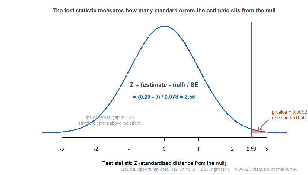
With the SE in hand we measure how far the observed estimate sits from the null value of “no effect” (\(0\)), in standard-error units:

\[Z = \frac{\text{estimate} - \text{null}}{\text{SE}} = \frac{0.20 - 0}{0.078} = 2.56.\]

This \(Z\) is the test statistic: the observed gap is \(2.56\) standard errors above zero. Mathematics (the Central Limit Theorem) guarantees that, for a statistic like this, the null distribution is approximately a smooth normal curve — so we no longer need to draw it by simulation. The p-value is the tail beyond \(Z = 2.56\) on that curve: \(p = 0.0052\). Compare:

Method	p-value
Week 11 simulation (1,000 shuffles)	\(\approx 0.006\)
Week 12 normal-model formula	\(0.0052\)

Two panels side by side. The left panel titled Week 11 simulation shows a histogram of simulated differences centered at zero with a red line at 0.20 in the right tail and the label p equals 0.006. The right panel titled Week 12 normal-model formula shows a smooth bell curve centered at zero with the right tail beyond 0.20 shaded, the formula Z equals 0.20 minus 0 over 0.078 equals 2.56, and the label p equals 0.0052. The two p-values are nearly identical. — A side-by-side comparison of the two methods on the opportunity-cost study. The left panel, labeled Week 11 simulation, is the histogram of 1,000 simulated differences with the observed 0.20 in the right tail and the note that 6 of 1,000 land there, giving p equals 0.006. The right panel, labeled Week 12 normal-model formula, is a smooth normal curve centered at zero with standard error 0.078; the same tail beyond 0.20 is shaded, and the test statistic Z equals 0.20 minus 0 over 0.078 equals 2.56 gives p equals 0.0052. The two p-values agree closely.

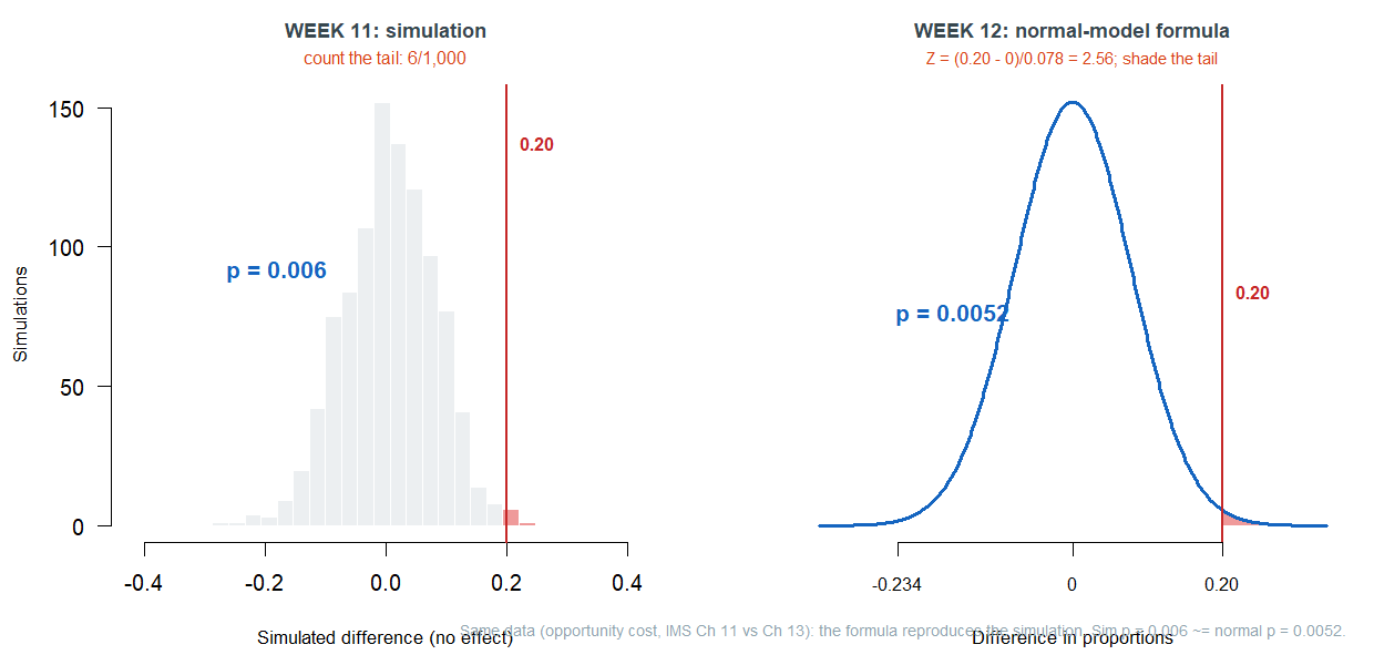
The two pictures are the same story told two ways. The simulation builds the null distribution; the formula assumes its shape is normal and reads the tail. When the assumption holds, they agree — and that agreement is the entire justification for the classical shortcut.

Monday, continued: null, test statistic, p-value as classical objects

Now the vocabulary, stated once and reused all week. A classical test has four pieces:

The null hypothesis \(H_0\): the skeptic’s “nothing is going on” (no effect, no difference, parameter equals some null value). For opportunity cost, \(H_0\): the reminder makes no difference (the true difference in proportions is \(0\)).
The alternative hypothesis \(H_A\): what we would conclude if the evidence is strong (an effect exists). It can be one-sided (a difference in a stated direction) or two-sided (a difference in either direction); two-sided is the cautious default.
The test statistic, \((\text{estimate} - \text{null})/\text{SE}\), which standardizes the result into “how many SEs from the null.” For proportions and large samples this is a \(z\); for means it is a \(t\) (next section).
The p-value, the area in the tail(s) of the model curve beyond the test statistic — the chance, if \(H_0\) were true, of a result this extreme.

We compare the p-value to a significance level \(\alpha\) (commonly \(0.05\)) and reject \(H_0\) when \(p < \alpha\). The traditional name for clearing that bar is statistically significant; IMS sometimes writes statistically discernible for the same idea, but we will say significant.

A bell-shaped standard normal curve centered at zero on a horizontal axis labeled test statistic Z. A red vertical line at 2.56 sits in the right tail and the area beyond it is lightly shaded, with an arrow labeling it the p-value equals 0.0052. Centered text reads Z equals estimate minus null over SE equals 0.20 minus 0 over 0.078 equals 2.56, and a note says the observed gap is 2.56 standard errors above no effect. — A standard normal curve for the opportunity-cost test statistic. The curve is centered at zero. A red vertical line marks Z equals 2.56, and the small tail to its right is shaded as the p-value of 0.0052. A centered annotation shows the test statistic equals estimate minus null over standard error, equals 0.20 minus 0 over 0.078, equals 2.56, describing the observed gap as 2.56 standard errors above no effect.

Monday’s honest footnote: when the shortcut is loose

The formula is an approximation, and approximations have limits. Take the medical-consultant case from last week: \(\hat p = 3/62 = 0.048\) complications against a national rate of \(10\%\). The normal-model test gives \(Z = (0.048 - 0.10)/0.038 = -1.37\) and a p-value of \(0.0853\). But last week’s simulation gave about \(0.1222\) — noticeably larger. The normal model is too optimistic here, because with only \(62\) surgeries and a small proportion the true null distribution is skewed, not the symmetric bell the formula assumes. The lesson cuts both ways: the formula usually reproduces the simulation (opportunity cost), but when the sample is small or the proportion is near \(0\) or \(1\), trust the simulation. The two methods agreeing is reassuring; the two methods disagreeing is a warning about the formula’s assumptions.

The standard error and the confidence interval

The same \((\text{estimate}, \text{SE})\) pair that powers a test also builds a confidence interval — the classical version of last week’s bootstrap interval. Instead of reading percentiles off a bootstrap distribution, we go a fixed number of standard errors out from the estimate:

\[\text{estimate} \pm z^\star \times \text{SE},\]

where \(z^\star = 1.96\) (about \(2\)) for \(95\%\) confidence, \(1.65\) for \(90\%\), and \(2.58\) for \(99\%\). The quantity \(z^\star \times \text{SE}\) is the margin of error. For the stent study, the estimated increase in 30-day stroke risk was \(0.090\) with \(\text{SE} = 0.028\), so

\[0.090 \pm 1.96 \times 0.028 = (0.035,\ 0.145).\]

We are \(95\%\) confident the true increase is between \(3.5\) and \(14.5\) percentage points. Because the interval lies entirely above zero, “no effect” is not a plausible value — the stent increased risk. That is the duality between tests and intervals: a \(95\%\) interval that excludes the null value corresponds to a two-sided test that rejects at \(\alpha = 0.05\), and an interval that contains the null corresponds to a test that fails to reject. The interval does double duty — it gives a decision and a set of plausible values, the two questions of inference in a single line.

Wednesday: reading a \(t\)-test and a proportion-test output

In practice you will rarely compute these by hand; you will read software output. Two small wrinkles first. For a proportion, the test statistic is a \(z\) and the curve is the normal — e.g., a payday-loan poll of \(n = 826\) with \(\hat p = 0.51\) tested against \(p_0 = 0.50\) gives \(Z = (0.51 - 0.50)/0.017 = 0.59\), a one-sided \(p = 0.2776\): nowhere near significant, so we fail to reject. For a mean, the SE must be estimated from the data’s own spread, which adds a little extra uncertainty, so we use a \(t\)-distribution instead of the normal. The \(t\) looks like the normal but with slightly thicker tails; the smaller the sample, the thicker, and for large samples the two are indistinguishable. Each \(t\) comes with degrees of freedom (df), roughly the sample size minus one — you read it off the output, you do not look it up in a table.

Here are two real outputs, annotated for reading:

Two mock software output boxes side by side. The left box headed One Sample t-test lists n equals 19, mean equals 4.40, s equals 2.30, SE equals 0.528, df equals 18, t-star equals 2.10 at 95 percent, and a 95 percent confidence interval 3.29 to 5.51, with red callouts pointing to the estimate and the plausible-values interval. The right box headed Welch Two Sample t-test lists nonsmoker n 100 mean 7.18 s 1.60, smoker n 50 mean 6.78 s 1.43, difference 0.40 pound, then t equals 1.54, df about 89.3, p equals 0.138, and a decision line that p greater than 0.05 means fail to reject. — Two annotated software t-test outputs. The left panel is a one-sample t for Risso’s dolphin muscle mercury: n equals 19, mean 4.40, s 2.30, standard error 0.528, df 18, t-star 2.10 for 95 percent, and a 95 percent confidence interval of 3.29 to 5.51, with the mean labeled the estimate and the interval labeled plausible values. The right panel is a two-sample Welch t-test for birth weight by maternal smoking: nonsmokers n 100 mean 7.18 s 1.60, smokers n 50 mean 6.78 s 1.43, difference 0.40 pound, t equals 1.54, df about 89.3, p equals 0.138, and the decision that since p exceeds 0.05 we fail to reject.

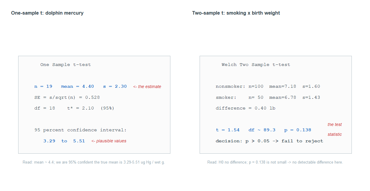
Read the left panel — a one-mean \(t\) for mercury in \(19\) Risso’s dolphins — as an estimation problem: the mean is \(\bar x = 4.4\) micrograms per gram, and the \(95\%\) interval \((3.29, 5.51)\) is the range of plausible values for the true mean. Read the right panel — a two-mean \(t\) comparing birth weights of babies born to nonsmokers versus smokers — as a test: the observed difference is \(0.40\) lb, \(t = 1.54\) on about \(89\) df, and \(p = 0.138\). Because \(0.138 > 0.05\) we fail to reject \(H_0\): in this sample there is no detectable difference. (Notice how the same machine handles one mean, two means, and a proportion — only the SE formula and the curve change.) The skill for the week is exactly this: find \(H_0\), read the estimate, the test statistic, the df, the p-value, and the CI, and write a conclusion in context — not just “reject” or “fail to reject.”

Friday: when a test goes wrong — Type I and Type II errors

A test ends in a yes/no decision about \(H_0\), and the truth is also yes/no, so there are exactly two ways to be wrong:

A two by two table. Rows are labeled the truth: H0 true, no effect, and HA true, real effect. Columns are labeled the decision: fail to reject H0 and reject H0. Top-left cell, H0 true and fail to reject, is correct. Top-right cell, H0 true and reject, is a Type I error, reject a true null, false alarm. Bottom-left cell, HA true and fail to reject, is a Type II error, miss a real effect, false reassurance. Bottom-right cell, HA true and reject, is correct and labeled power. Side notes say alpha is the long-run Type I error rate and power is the chance of catching a real effect. — A two-by-two decision table titled the two ways a hypothesis test can be wrong. The rows are the truth, H0 true meaning no effect and HA true meaning a real effect. The columns are the decision, fail to reject H0 and reject H0. The cell for H0 true and reject is a Type I error, rejecting a true null, a false alarm. The cell for HA true and fail to reject is a Type II error, missing a real effect, a false reassurance. The other two cells are correct decisions; the reject-when-HA-true cell is labeled power. A side note says the significance level alpha is the long-run Type I error rate.

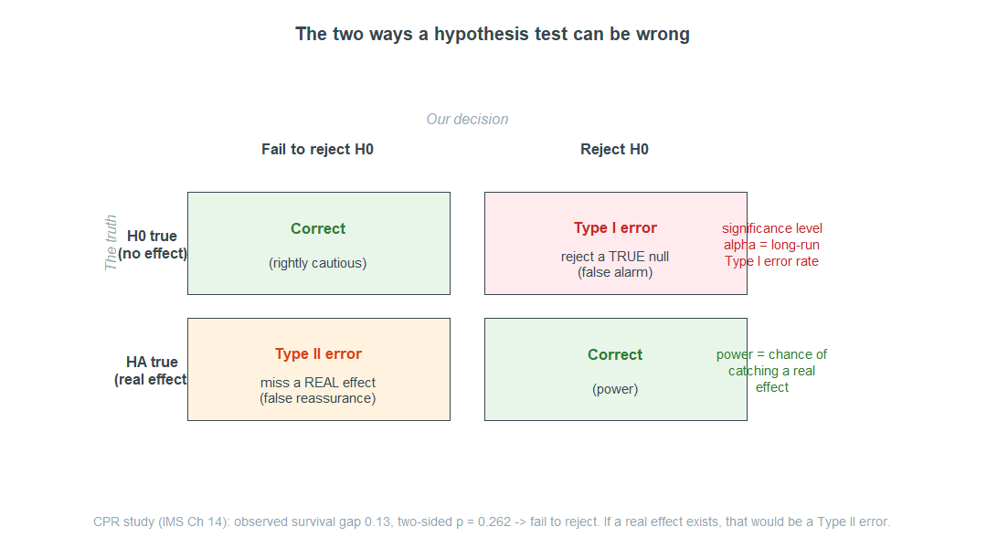
A Type I error is rejecting a true null — a false alarm, declaring an effect that isn’t there. A Type II error is failing to reject when the alternative is actually true — a missed real effect. The connection to the significance level is exact: \(\alpha\) is the long-run Type I error rate. Choosing \(\alpha = 0.05\) means accepting that, when nothing is going on, we will cry “effect!” about \(5\%\) of the time. If a false alarm is costly we set \(\alpha\) smaller (\(0.01\) or \(0.001\)); if missing a real effect is costlier we may allow a larger one. The two errors trade off — squeezing one tends to inflate the other — which is why you cannot drive both to zero.

The flip side of a Type II error is power: the probability of correctly rejecting \(H_0\) when there really is an effect. Power rises with a larger true effect and a larger sample size — bigger signals and more data are both easier to detect. (We treat power conceptually only; there is no formula to memorize here.)

A worked decision: the CPR study compared survival after a blood thinner. Survival was \(11/50 = 0.22\) in the control group and \(14/40 = 0.35\) in the treatment group, a difference of \(0.13\) in favor of treatment. Because the researchers had no prior direction, they ran a two-sided test and got a p-value of \(0.262\) — far above \(0.05\) — so they failed to reject \(H_0\): no convincing evidence of a survival effect. That conclusion is honest, but note the risk: if the thinner truly helps, “fail to reject” would be a Type II error, a missed effect a larger study might catch. “No significant difference” is never the same as “no difference.”

One discipline this makes vivid: decide your hypotheses before you see the data. Peeking and then switching a two-sided test to whichever one-sided version “works” quietly doubles your Type I error rate from \(5\%\) to \(10\%\) — you have given chance two bites at the apple.

A note on regression inference (closing the Week 9 loop)

Back in Week 9 we read a regression output and greyed out the “Std. Error / \(t\) / p-value” columns, promising to return. This is the return, and it is short: those columns are exactly this week’s idea applied to a slope. Each slope estimate has a standard error, a test statistic of the same \((\text{estimate} - \text{null})/\text{SE}\) form (with a null value of \(0\), meaning “this predictor has no association with the outcome once the others are held constant”), a p-value, and a confidence interval. So a slope’s p-value answers the familiar question — could this association be chance? — and its CI gives plausible values for the slope. That is all you need to read a regression’s inference columns; the machinery for computing them is a later, more-advanced topic and is not part of this course.

Common mistakes

“The p-value is the probability the null is true.” Still no — it is the probability of data this extreme if \(H_0\) is true. The classical curve does not change that.
“Fail to reject means the null is true.” It means not enough evidence against it. The CPR study failed to reject, but a real effect could still exist (a Type II error).
“Statistically significant means the effect is large or important.” A test rules out chance; it says nothing about size. With a big enough \(n\), a trivial effect can be significant.
“Use a \(z\) for everything.” Means use a \(t\) (estimated SE, thicker tails); proportions use a \(z\). Read which one the output reports.
“Pick the hypothesis direction after seeing the data.” That inflates the Type I error rate. Set \(H_0\) and \(H_A\) first.
“The confidence interval and the test are different analyses.” They are two faces of one thing: an interval excluding the null value matches a test that rejects.

What you should be able to do by Friday

By the end of Week 12 you should be able to:

state a null and alternative hypothesis for a study, and tell one-sided from two-sided;
explain the test statistic \((\text{estimate} - \text{null})/ \text{SE}\) as “how many standard errors from the null,” and the p-value as a tail area of the model curve;
read a proportion \(z\)-test, a one-mean \(t\), and a two-mean \(t\) output — finding \(H_0\), the estimate, the statistic, the df, the p-value, and the CI — and conclude in context;
build and read a confidence interval as \(\text{estimate} \pm z^\star \times \text{SE}\), and use the test–interval duality;
name and distinguish Type I and Type II errors, explain \(\alpha\) as the Type I error rate, and describe power conceptually;
explain why the classical formula reproduces last week’s simulation — and when (small \(n\), skew) it may not.

Assignments this week

Monday check. A short in-class concept check on stating the null and identifying the test statistic (and matching the formula to last week’s simulation idea). Plan for about 3–5 minutes. Sheet: Week 12 Monday exit ticket.
Wednesday check. A short application reading a \(t\)-test or proportion-test output: state \(H_0\), read the p-value and CI, and conclude in context. Plan for about 8–12 minutes. Sheet: Week 12 Wednesday exit ticket.
🔒 Friday quiz — handled through Blackboard or in class as directed. The quiz prompt is not posted here. Timing and submission details live in Blackboard.
🔒 Homework 6 (biweekly, Weeks 11–12) — posted and submitted through Blackboard. It spans last week and this one, including a bridge problem that runs one case study by both simulation and formula; due near the start of the following week.

Reuse

CC BY-SA 3.0.