Week 9 — Multiple and logistic regression, by interpretation

MATH 21003 · Introduction to Statistical Methods · Fall 2026 · Week 9 (Oct 19–23, 2026)

Why this week matters

Week 8 fit a line with one predictor and taught us to read its slope. The trouble is that the world rarely hands us one predictor at a time. A statin user is also, on average, older. A loan with a past bankruptcy is also, on average, a loan with other red flags. When two explanations are tangled together — exactly the confounding we worried about in Week 6 — a single-predictor slope can tell a misleading story.

This week we add more predictors to the model at once and learn to read what each one says with the others held constant. That one phrase, “holding the other variables constant,” is the whole point of the week. It turns the Week 6 intuition — “what else could explain this?” — into something we can actually read off a model. We close by extending the same reading to a yes/no outcome with logistic regression, where the model predicts a probability instead of a number.

A note on the rhythm. Monday introduces multiple regression and the “holding constant” reading. Wednesday practices it on a harder case — comparing an unadjusted model to an adjusted one and explaining why a number moved. Friday’s quiz checks that you can read an adjusted model in a new scenario and read the direction of a logistic model. As always, the small midweek work is the most reliable preparation.

Adding a predictor

A simple regression predicts an outcome from one predictor. A multiple regression predicts the same outcome from several predictors at once:

\[\hat{y} = b_0 + b_1 x_1 + b_2 x_2 + \cdots + b_k x_k.\]

Each predictor \(x_j\) gets its own coefficient \(b_j\). The equation still produces a single predicted value \(\hat{y}\) — you plug in a value for each predictor and add up the pieces, exactly as before.

The IMS textbook models the interest rate on a set of about 10,000 loans. Using seven predictors at once, the fitted model is

\[ \begin{aligned} \widehat{\text{rate}} = \;& 1.89 + 1.00\,(\text{income: source-verified}) + 2.56\,(\text{income: verified}) \\ & + 0.02\,\text{debt-to-income} + 4.90\,\text{credit-utilization} \\ & + 0.39\,\text{past-bankruptcy} + 0.15\,\text{loan-term} + 0.23\,\text{credit-checks}. \end{aligned} \]

It looks busier than a single-predictor line, but it is read the same way: each coefficient is a slope, and the model predicts one number. What changes — and what makes this week worth a week — is what each of those slopes now means.

“Holding the other variables constant”

Here is the central idea. In a multiple regression, a coefficient \(b_j\) tells you the average change in \(\hat{y}\) for a one-unit increase in \(x_j\) while every other predictor stays fixed. The standard phrases for this are holding the other variables constant and after adjusting for the other variables. They mean the same thing.

Take the credit-checks coefficient, \(0.23\). Reading it in plain English: among loans that are otherwise the same — same income verification, same debt-to-income, same credit utilization, same bankruptcy history, same term — each additional credit inquiry is associated with a predicted interest rate about \(0.23\) percentage points higher, on average. The phrase “otherwise the same” is doing all the work. It is what separates a multiple-regression coefficient from a one-variable slope.

Why does that separation matter? Because the same predictor can have a different slope depending on what else is in the model. In a single-predictor model, a past bankruptcy is associated with a rate about \(0.74\) points higher. In the seven-predictor model above, the bankruptcy coefficient is only \(0.39\). Nothing about the loans changed; the difference is that the larger model has already accounted for the other things that tend to travel with a bankruptcy (higher credit utilization, more credit checks). Once those are held constant, the part of the rate that bankruptcy alone explains is smaller. The single-predictor \(0.74\) was partly standing in for its companions.

This is the same move we make all week, so it is worth saying once more, carefully: an adjusted coefficient is the predictor’s association with the outcome after the model has subtracted off what the other predictors can explain. It is still an association, not a proven cause — but it is a much more honest association than the one-variable version.

Categorical predictors

Not every predictor is a number. Income verification in the loans data is a category with three levels: not verified, source verified, and verified. A regression handles a categorical predictor by choosing one level as the reference and reporting each other level relative to it. Fit on its own, income verification gives:

Verification level	Predicted rate
Not verified (reference)	11.10%
Source verified	12.52%
Verified	14.35%

The reference level, not verified, is built into the intercept: \(11.10\%\). The other two numbers are read as differences from the reference. Source-verified loans run about \(1.42\) points higher than not-verified (\(11.10 + 1.42 = 12.52\)); verified loans run about \(3.25\) points higher (\(11.10 + 3.25 = 14.35\)). This is the two-level indicator idea from the end of Week 8, now generalized: a category with \(L\) levels enters the model as \(L-1\) comparisons, each one measured against the reference. You read each coefficient as “this level versus the reference, on average.”

When adjustment changes the story

The reason “holding constant” earns a whole week is that adjustment can change a conclusion, not just shrink a number. This is the Week 6 confounding lesson, now told with coefficients.

The ISLBS textbook studies cognitive function in the PREVEND study: 500 Dutch adults whose thinking was scored on a 0–175 cognitive test (the RFFT). One question was whether statin use is associated with cognitive score. Fit by itself, the statin coefficient is about \(-10.05\) — statin users score about ten points lower, which reads alarmingly like “statins go with worse cognition.”

But statin users are, on average, older, and older adults score lower on this test for reasons that have nothing to do with statins. Age is a confounder. Watch what happens to the statin coefficient as we add predictors to hold age (and then education and prior cardiovascular disease) constant:

A line chart with three points connected left to right. The vertical axis is the statin coefficient on cognitive score in test points. The first point, labeled Unadjusted, is at about negative 10.05, well below a dashed zero line. The second point, labeled plus Age, is at about positive 0.85, just above zero. The third point, labeled plus Age, Education, prior CVD, is at about positive 4.69. The points are connected by a rising line that crosses zero between the first and second point. — A coefficient path. The statin coefficient on cognitive score starts at about negative 10.05 when unadjusted, jumps to about positive 0.85 once age is held constant, and rises to about positive 4.69 once age, education, and prior cardiovascular disease are all held constant. A dashed horizontal line marks zero; the unadjusted point sits well below it and the adjusted points sit above it. The figure shows the apparent harm disappearing after adjustment.

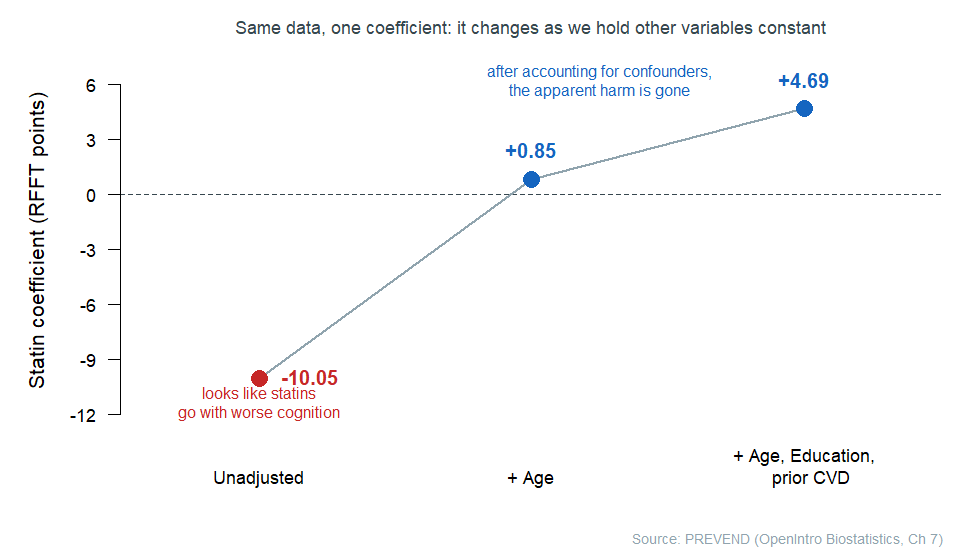
The \(-10.05\) was almost entirely age in disguise. Once age is held constant the coefficient is essentially zero (about \(+0.85\)), and with a few more confounders held constant it is mildly positive (\(+4.69\)) — no evidence of harm at all. Same data, same statin variable; the story flips because the model now holds the confounders constant. (The loans bankruptcy coefficient told a quieter version of the same tale: \(0.74\) alone, \(0.39\) adjusted.)

This is what multiple regression is for in this course: it is the engine behind the Week 6 phrase “after accounting for.” It does not turn an observational association into proof — statin users could still differ in some way the model did not measure — but it lets us ask the adjusted question instead of the naive one.

Reading the output, and how much the model explains

In practice you will not fit these models by hand; you will read them from a software output table. The habit to build this week is to read one column — the estimates — and ignore the rest for now.

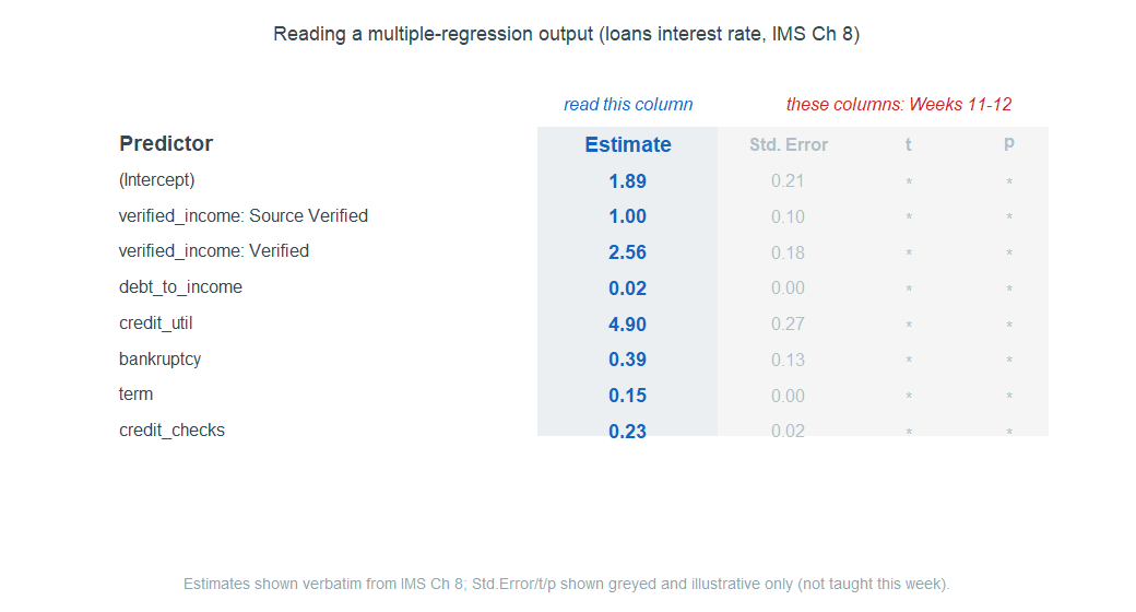
A regression output table. Predictor names run down the left. The Estimate column is shaded and labeled read this column, listing one number per predictor. To its right, three columns labeled Standard Error, t, and p are greyed out with a note saying these columns are for Weeks 11 to 12. — An annotated regression output table for the loans model. The left column lists the predictors. A highlighted middle column, labeled “read this column,” shows the estimate for each predictor: intercept 1.89, source-verified 1.00, verified 2.56, debt-to-income 0.02, credit utilization 4.90, bankruptcy 0.39, term 0.15, credit checks 0.23. Three further columns headed Std. Error, t, and p are greyed out and flagged “these columns: Weeks 11-12.”

Real output tables report several more columns next to each estimate — a standard error, a \(t\) value, a \(p\)-value. We ignore those columns this week. They belong to inference, which asks whether a coefficient is distinguishable from zero in the larger population, and that is a Week 11–12 topic. For now: find the estimate column, read the estimates, and leave the rest greyed out.

One summary number is worth reading: adjusted \(R^2\). Plain \(R^2\) is the share of the variation in the outcome the model captures — the same idea as Week 8, where \(R^2 = r^2\). With several predictors, plain \(R^2\) has a flaw: it can only go up when you add a predictor, even a useless one. Adjusted \(R^2\) applies a small penalty for each extra predictor, so it only rises when a predictor genuinely helps. For the loans model, \(R^2\) is about \(0.259\) and adjusted \(R^2\) is about \(0.258\) — the model captures roughly a quarter of the variation in interest rate. You read adjusted \(R^2\) as a number, the same way; you do not need its formula.

That penalty hints at a caution worth one sentence: more predictors is not automatically better. Two predictors that carry nearly the same information (say, two almost-identical measures of credit risk) can muddy each other’s coefficients, a situation called multicollinearity. You do not need to diagnose it this week — just know that piling in overlapping predictors can make individual coefficients hard to interpret, which is why a smaller, sensible model is often the more honest one.

Yes/no outcomes: logistic regression by interpretation

So far the outcome has been a number. Often the outcome is yes/no: does a loan default, does a patient have the condition, does a screened resume get a callback. For a yes/no outcome we use logistic regression, and in this course we read it by interpretation only.

Here is the one structural fact you need. A yes/no outcome cannot be predicted as a raw number — a “probability of 1.3” is meaningless — so logistic regression predicts the probability that the answer is “yes,” and it is built so that this predicted probability always lands between 0 and 1. Behind the scenes the model does its arithmetic on a transformed scale to guarantee that; you will never have to manipulate that scale. You read two things: the direction of each predictor, and the predicted probability the model produces.

A curve on axes where the horizontal axis is temperature in degrees Fahrenheit from 50 to 85 and the vertical axis is predicted probability from 0 to 1. The curve starts near 0.7 at 50 degrees and decreases in a smooth S-shape toward 0 by about 80 degrees. Several points along the curve mark the model's estimated probabilities. An arrow indicates that higher temperature corresponds to lower predicted probability. — A logistic regression curve. Temperature in degrees Fahrenheit is on the horizontal axis; the predicted probability of O-ring damage is on the vertical axis, running from 0 to 1. The curve is high (near 0.7) at low temperatures and falls in an S-shape toward 0 as temperature rises, with the model’s estimated probabilities marked as points. A red arrow notes that higher temperature goes with lower predicted probability. A note observes the curve only ever predicts a probability between 0 and 1.

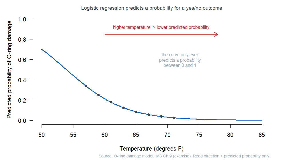
The figure shows a classic example: the modelled probability of O-ring damage on a rocket launch as a function of outside temperature. Direction first — the curve falls as temperature rises, so higher temperature goes with a lower predicted probability of damage. Predicted probability second — at a cold \(57°\)F the model predicts about a \(0.34\) chance of damage; by a warm \(71°\)F it predicts about \(0.02\). That is the whole reading: which way a predictor pushes the chance, and what chance the model gives for a particular case.

Everything from the first half of the week carries over. A logistic model can have several predictors, and each one is read holding the others constant — the same adjustment idea, now phrased as “raises or lowers the predicted probability, all else equal.” What we are not doing this week: we are not fitting the model by hand, not working with its transformed scale, not computing odds, and not reading any inference columns. Direction and predicted probability are enough.

Common mistakes

“An adjusted coefficient proves causation.” It does not. Adjustment removes the influence of the confounders you measured and included. An unmeasured confounder can still be hiding. An adjusted association is more honest than a crude one, not a proof.
“A coefficient means the same thing in every model.” No — it depends on what else is in the model. The bankruptcy slope was \(0.74\) alone and \(0.39\) adjusted. Always read a coefficient as “holding these particular other variables constant.”
“The intercept is the prediction when everything is zero, so it’s meaningful.” Usually it is not. If “all predictors equal zero” is impossible or outside the data (a loan with zero term?), the intercept is just scaffolding.
“A bigger model with more predictors is a better model.” Not automatically. Adjusted \(R^2\) penalizes useless predictors, and overlapping predictors can muddy each other. Smaller and sensible often wins.
“Logistic regression predicts yes or no.” It predicts a probability of yes, between 0 and 1. Turning that probability into a decision is a separate step we are not taking here.
“Read the whole output table.” Not this week. Read the estimate column; the standard-error, \(t\), and \(p\) columns are Weeks 11–12.

What you should be able to do by Friday

By the end of Week 9 you should be able to:

read a multiple-regression equation and use it to produce a predicted value;
interpret a single coefficient holding the other variables constant, in real units and with the on average qualifier;
read a categorical predictor against its reference level;
explain why a coefficient can change between an unadjusted and an adjusted model, and connect that to Week 6 confounding;
read adjusted \(R^2\) as the share of variation the model captures, and state the one-sentence caution that more predictors is not automatically better;
find and read the estimate column of a regression output, and say why the inference columns are set aside until later;
read a logistic regression by direction and predicted probability for a yes/no outcome, without touching its underlying scale.

Assignments this week

Monday check. A short concept check on reading a coefficient “holding the other variables constant.” Aim for about 3–5 minutes in class. Sheet: Week 9 Monday exit ticket.
Wednesday check. A short application comparing an unadjusted and an adjusted regression output and explaining why a coefficient moved. Aim for about 8–12 minutes in class. Sheet: Week 9 Wednesday exit ticket.
🔒 Friday quiz — handled through Blackboard or in class as directed. The quiz prompt is not posted here. Exact timing and submission details live in Blackboard.
🔒 Homework 5 (biweekly, Weeks 9–10) — posted and submitted through Blackboard. It spans this week and next; due near the start of Week 11.

Reuse

CC BY-SA 3.0.